Note: This post has a lot of javascript graphs, but if you’re using a feed reader or have javascript turned off you’ll just get basic tables. Sorry about that.

With that out of the way: I’m going to assume that if you’re reading this you’ve already read Part 1. As such, I’m just going to dive right back in where I left off.

Calculating the Per Business F1 on the Fly

Having now calculated the per business F1 at the end of the training run, I realised it would be useful (or at least interesting) to be able to see how it was changing during training. The per photo F1 makes for a decent heuristic, but isn’t guaranteed to actually correlate with the per business F1, which is what I actually care about.

I hit another snag here with the the fast.ai library. At the end of each epoch, the metrics supplied by the user are calculated using the same batch size as training. The results for each batch are then averaged, and this is what is shown to the user.

That’s a problem for calculating the per business F1, as the entire dataset is needed to build the per business predictions. As a smaller and less obvious problem: it also means that the per photo F1 which is displayed at the end of the epoch will be even more inflated than I thought. This is because rather than finding the best threshold for the entire data set, a more specialised threshold will be found for each batch. It’s overfitting, essentially. The premature optimisation of the machine learning world.

I could solve both problems if I could collate the per photo predications before calculating the F1. If I had access to state which persisted between batches, I could use something like the method below to collate the predictions and target values.

def collate(preds, targs, data):
  multiplier = 1.0
  if preds.shape[0] != len(photo_idx_to_val_biz_idx):
    if data['preds'] is None:
      data['preds'] = preds
      data['targs'] = targs
      # The dataset is incomplete.
      return 0, None, None
    # Append the data to the known data.
    data['preds'] = torch.cat([data['preds'], preds])
    data['targs'] = torch.cat([data['targs'], targs])
    if data['preds'].shape[0] != len(photo_idx_to_val_biz_idx):
      # The dataset is incomplete.
      return 0, None, None
    # The dataset is complete.
    # See below for an explanation of the multiplier.
    multiplier = len(photo_idx_to_val_biz_idx) / preds.shape[0]
    preds = data['preds']
    targs = data['targs']
    data['preds'] = None
    data['targs'] = None
  return multiplier, preds, targs

That’s all well and good, but the metric calculations are supplied to the fast.ai library as a pure function, which is then run without additional state or context. Except… this is Python, and calling something a “pure” function is a sign, not a cop. Functions in Python are first class objects, and objects in Python have arbitrarily assignable state. So there is a way around this problem…

Warning: If the Python code I admitted to using elsewhere in these posts bothers you, that below will almost certainly bother you even more. And it should. It’s a horrible hack, and nothing like it should ever get anywhere near a production environment. It should never even get near the critical path of a non production environment. But still. I’m not using it for either of those things.

def f1_biz_avg(preds, targs, start=0.24, end=0.50, step=0.01):
  # Collate the predictions and targets, using persistent
  # state attached to this function.
  multiplier, preds, targs = collate(preds, targs, f1_biz_avg.data)

  # A multiplier of 0 means that collation is incomplete.
  if multiplier == 0.0:
    return 0
    
  # Convert the per photo values to per business values.
  biz_preds, biz_targs = photo_to_biz(preds, targs, True)

  # Ignore warnings.
  with warnings.catch_warnings():
    warnings.simplefilter("ignore")

        # Find the threshold which yields the best F1.
    mapping = {th : f1_score(biz_targs, (biz_preds > th), average='samples')
           for th in np.arange(start,end,step)}
    th = max(mapping.keys(), key=mapping.get)

    # Return the best F1, scaled so that the fast.ai library
    # will average it with the 0's to get the correct value. 
    return mapping[th] * multiplier

# Initialize the persistent state.
f1_biz_avg.data = {'preds': None, 'targs': None}

This works around two issues:

1. Collating the predications before calculating the F1;
2. Scaling the output of the final batch so that when it’s averaged with the zeros returned for the other batches the correct value results.

I’ll say it again: all of this is a horrible hack. I’m ashamed of it. I worry that if anyone who works for my employer sees this, I might be fired. And yet...

This is how the per photo F1 compares to the business F1 over the course of the training schedule:

As you can see the per business F1 is consistently higher than the per photo, but less stable. The latter makes sense, given that the model is being trained against the individual photos, not the business. The former was a little surprising to me. I assume the mixed signals start to cancel each other out when you average the predications together.

Comparing Different Architectures

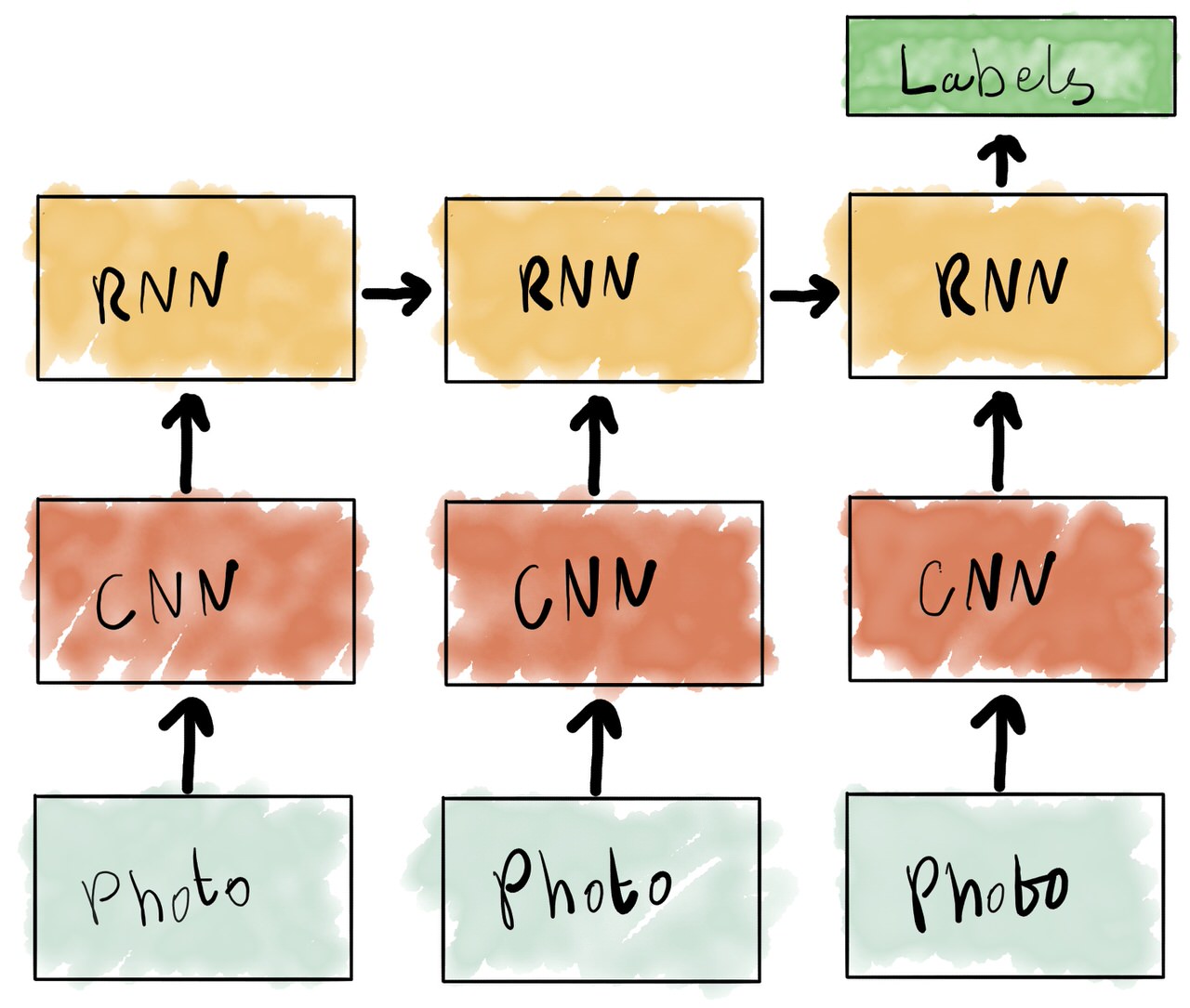
An F1 of 0.7845 was actually pretty close to my original goal, but not quite there. The obvious next step was to try the same approach with a more advanced model. I also thought it might be interesting to compare the performance of a few different CNN architectures for my own information. So next I ran the exact same schedule, but using the ResNet-50 and ResNext-50 CNN architectures.

One advantage ResNext-50 did have is that it trained more quickly. Stupidly, I didn’t record the training time for each architecture. I trained ResNet-34 over the course of a day. I’d say that ResNet-50 look about half as long again to train as ResNet-34^[1]. ResNext-50 seemed like it took about halfway between the two. But that could be my imagination. Next time I should actually record the timings…

Be that as it may, my initial goal was to achieve an F1 score of at least 0.8 against the validation set. 0.8082 is (just barely) higher than that, so: mission accomplished, I guess.

Right?

Trying Class Specific Thresholds

At this point I started to realise a few things which would have been obvious at the top if I had more experience. Firstly, after I started writing this post I realised it might be interesting to graph the proportion of businesses which belong to each class. For your convenience (and in the interest of making the following charts readable on mobile), here are the class names again:

0. Good for lunch;
1. Good for dinner;
2. Takes reservations;
3. Outdoor seating;
4. Restaurant is expensive;
5. Has alcohol;
6. Has table service;
7. Ambience is classy;
8. Good for kids.

And here is a graph of their proportions:

Following on from this, I started to wonder whether my system was doing better on some classes rather than others. Which is when the obvious thought arrived: I was using the same threshold for each class, but I had no reason to assume that the sensitivity was the same. I could probably get better results by using different thresholds for each class.

I ran the following code against the inference output for the validation set to find the best individual threshold for for each class:

def per_class_threshholds(preds, targs, start=0.04, end=0.50, step=0.001):

  # Initialize the per class threshholds to 0.
  thresholds = np.zeros((preds.shape[1]))

  # Ignore warnings.
  with warnings.catch_warnings():
    warnings.simplefilter("ignore")
  
    # Iterate 10 times, trying to improve the thresholds each
    # time.
    # Note: This is overkill, but runs quickly enough not to matter.
    # Some CPU time could be saved by stopping once the F1 is no 
    # longer improving.
    for _ in range(10):
      # Try to improve the threshold for each class in turn.
      for i in range(0, thresholds[0]):
        best_th = 0.0
        best_score = 0.0
        for th in np.arange(start, end, step):
          thresholds[i] = th
          score = f1_score(targs, (preds > thresholds), average='samples')
          if score > best_score:
            best_th = th
            best_score = score
        thresholds[i] = best_th

  return thresholds

Running this for each of three architectures individually gave me the per class F1 scores. You can see them in the graph below, which I’ve foreshortened to emphasise the differences in performance:

There’s actually more variation than I was expecting. Firstly between the per class scores. There’s some correlation with the per class proportions above, but not for every class. Accounting for that effect, “Good for lunch” and “takes reservations” appear to be the hardest classes to detect.

Secondly the best architecture is not consistent across the classes. ResNet-34 is actually a bit of a dark horse when it comes to detecting establishments which open for lunch. Who knew?

Speaking of ideas which occur to you after the fact: I’m willing to bet that the time stamp of the photo is probably a pretty solid signal for the “good for lunch” class.

At this point I didn’t trust the overall F1 scores these thresholds gave me against the validation set. It was time run against the test set, submit to Kaggle, and find out what my real score was. I did this for each of the architectures, and also built an ensemble output by using the predictions of the architecture which got the best score for each class.

Having run inference on the test data, I used the following code to build per business predications^[2] and generate the formatted output.

predications = # The per photo predictions.
test_photo_to_biz = f'{PATH}/test_photo_to_biz.csv'
test_photo_to_biz_data = pd.read_csv(test_photo_to_biz)

# Gather the individual business IDs, and the image counts
# for each business.
biz_counts = {}
for biz_id in test_photo_to_biz_data.business_id:
  biz_counts.setdefault(biz_id, 0)
  biz_counts[biz_id] += 1
biz_ids = list(biz_counts.keys())
biz_idxs = {biz_ids[i] : i for i in range(len(biz_ids))}

# Extract the photo IDs in order from the test image file names.
images_in_order = [v[9:-4] for v in learn.data.test_ds.fnames]
photo_idxs = {int(images_in_order[i]) : i for i in range(len(images_in_order))}

# Convert the per photo predictions to per business predictions.
biz_preds = np.zeros((len(biz_ids), preds2.shape[1]))
for i in range(test_photo_to_biz_data.shape[0]):
  photo_id = test_photo_to_biz_data.photo_id[i]
  photo_idx = photo_idxs[photo_id]
  photo_preds = predications[photo_idx, :]
  
  biz_id = test_photo_to_biz_data.business_id[i]
  biz_idx = biz_idxs[biz_id]
  biz_count = biz_counts[biz_id]
  
  biz_preds[biz_idx, :] += photo_preds * (1.0 / biz_count)

# Convert the predications into booleans.
biz_cls = preds > threshholds

# Convert the booleans into lists of matched classes.
classes = []
for i in range(biz_cls.shape[0]):
  biz_cls_biz = biz_cls[i, :]
  biz_classes = " ".join([str(i) for i in range(preds_cls.shape[1]) if biz_cls_biz[i]])
  classes.append(biz_classes)

# Build a pandas data frame with the business IDs and
# matched classes.
data = np.array(list(zip(biz_ids, classes)), order = 'F')
output = pd.DataFrame(data=data, columns=['business_id', 'labels'])
# Write the data frame out to a CSV files.
csv_fn=f'{PATH}tmp/sub_{f_model.__name__}.csv'
output.to_csv(csv_fn, index=False)
# Display a link to the CSV file.
FileLink(csv_fn)

The code used to build the ensemble is left as an exercise for the reader. Obviously this is for educational purposes. Not just because I don’t want you to see my code and possibly judge me more harshly than you already do for the other code in this post. Ahem.

So, without further ado, here are the final scores against the public and private leaderboards for the competition: