Simplifying the Landscape

At the end of the last post I wrote about the actual implementation of my Clockwork Aphid project, I said the next step was going to be display simplification. At that point I'd generated a few landscapes which were just starting barely starting to test the limits of my computer, though they were nothing like the size or complexity I had in mind. That said, it was looking at landscapes containing 1579008 polygons and it was obvious that not all of these needed to be put on screen. Moreover, because my landscapes are essentially made up of discrete samples (or nodes): I needed to reduce the number of samples which were displayed to the user, otherwise my performance was really going to tank as the landscapes increased in size.
Shamus Young talked about terrain simplification some time ago during his original terrain project. This seemed as good a place as any to start, so I grabbed a copy of the paper he used to build his algorithm. I didn't find it as complicated as it appears he did, but this is probably because I'm more used to reading papers like this (I must have read hundreds during my PhD, and even wrote a couple), so I'm reasonably fluent in academicese. It was, as I suspected, a good starting point, though I wouldn't be able to use the algorithm wholesale as it's not directly compatible with the representation I'm using. Happily, my representation does make it very simple to use the core idea, though.
If you remember, my representation stores the individual points in a sparse array, indexed using fractional coordinates. This makes it very flexible, and allows me to use an irregular level of detail (more on that later). Unlike the representation used in the paper, this means a can't make optimisations based on the assumption that my data is stored in a regular grid. Thankfully, the first stage of the simplification algorithm doesn't care about this and examines points individually. Also thankfully, the simplification algorithm uses the same parent/child based tessellation strategy that I do.
The first step is decide which points are "active". This is essentially based on two variables:
- The amount of "object space error" a point has (i.e. how much it differs from its parents);
- The distance between the point and the "camera".
A local constant is also present for each point:
- The point's bounding radius, or the distance to its furthest child (if it has children);
I'm not sure if I actually need this last in my current implementation (my gut says no, I'll explain why later), but I'm leaving it in for the time being. Finally, two global constants are used for tuning, and we end up with this:

Where:
- i = the point in question
- λ = a constant
- εi = the object space error of i
- di = the distance between i and the camera
- ri = the bounding radius of i
- τ = another constant
This is not entirely optimal for processing, but a little bit of maths wizardry transforms this like so:

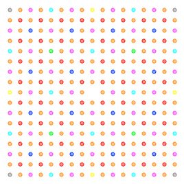
This looks more complicated, and it's less intuitive to see what it actually does, but from the point of view of the computer it's a lot simpler, as it avoids the square root needed to calculate the distance between the point and the camera. Now we get to the fun part: diagrams! Consider the following small landscape, coloured as to the granularity of each of the points (aka the distance to the node's parents, see this post):
Next, we'll pick some arbitrary values for the constants mentioned above (ones which work well for explanatory purposes), and place the viewpoint in the top left hand corner, and we end up with this the following active points (inactive points are hidden):

Now, we take the active points with the smallest granularity, and we have them draw their polygons, exactly as before, which looks like this:

When we come to draw the polygons of the next highest granularity you'll see that we have a problem, though. The previous set of polygons have encroached on their territory. To avoid this, each node informs its parents that it is active and then the parent doesn't draw any polygons in the direction of its active children. If we add in the polygons drawn by the each of the other levels of granularity, we now end up with this:
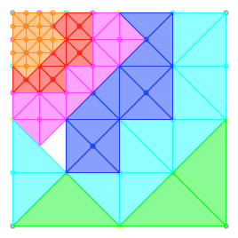
Oh no! There's a hole in my landscape! I was actually expecting that my simplistic approach would lead to more or less this result, but it was still a little annoying when it happened. If I was a proper analytical type I would next have sat down and worked over the geometry at play here, then attempted to find a formulation which would prevent this from happening. Instead, though, I stared at it for a good long while, displaying it in various different ways, and waited for something to jump out at me.
Eventually it did, and thankfully it was a very simple rule. Each parent stores a list of the directions in which it has active children in order to prevent overdrawing (as mentioned above). The new rule is that a node is also considered active if this list is non-empty. With this addition, our tessellated landscape now look alike this:
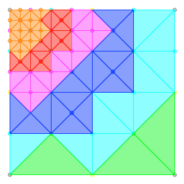
Presto! A nice simple rule which fills in all of the gaps in the landscape without any over or under simplification, or any overdrawing. I suspect this rule also negates the need for the bounding radius mentioned above, though I have not as yet tested that thought. To recap, we have three simple rules:
- A node is active if the object space error/distance equation says it is;
- A node is active if any of its children are active;
- Polygons are tessellated for each active point, but not in the direction of any active children.
But what does this look like in actual eye poppingly 3D landscapes? Well, here's an example, using the height based colouring I've used before:
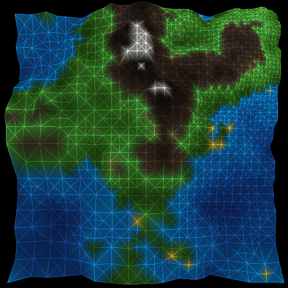
I'm quite pleased with this, though what I'm doing here is still quite inefficient and in need of some serious tuning. There are a couple of further simplification tricks I can try (including the next step from the (paper) paper). More to come later. Honest.